Slice sampling
This post is a demonstration of slice sampling. The goal is to sample from a target distribution f(x). A slice variable, u, is added where the joint density is p(u,x) = I(0<u<f(x)) which maintains the marginal distribution for x. A Gibbs sampler is constructed with the following steps
-
u x ~ Unif(0,f(x)) -
x u ~ Unif over the set A where A={x:u<f(x)}.
The rest of this post considers situations where A is relatively easy to find, e.g. monotone functions f(x) over the support of x and unimodal functions.
Here is a generic function (okay, it probably isn’t that generic, but it works for the purpose below) to implement slice sampling. It takes a number of draws n, an initial x, the target density, and a function A that returns the interval A, so only unimodal targets supported. The function returns the samples x and u (for demonstration).
# Slice sampler
slice = function(n,init_x,target,A) {
  u = x = rep(NA,n)
  x[1] = init_x
  u[1] = runif(1,0,target(x[1])) # This never actually gets used

  for (i in 2:n) {
    u[i] = runif(1,0,target(x[i-1]))
    endpoints = A(u[i],x[i-1]) # The second argument is used in the second example
    x[i] = runif(1, endpoints[1],endpoints[2])
  }
  return(list(x=x,u=u))
}
In this first example, the target distribution is Exp(1). The set A is just the interval (0,-log(u)) where u is the current value of the slice variable.
# Exponential example
set.seed(6)
A = function(u,x=NA) c(0,-log(u))
res = slice(10, 0.1, dexp, A)
x = res$x
u = res$u| Here is a demonstration of a single step of the slice sampler. Given a coordinate (u,x), the sampler first draws from u | x which is equivalent to slicing the density vertically at x and drawing uniformly on the y-axis from the interval where u<f(x) and then draws x | u which is equivalent ot slicing the density horizontally at u and drawing uniformly on the x-axis from the interval where u<f(x). |
i = 2
curve(dexp,0,2,ylim=c(0,1))
points(x[i],u[i],pch=19)
segments(x[i], 0, x[i], dexp(x[i]), col="gray")
arrows(x[i], u[i], x[i], u[i+1], length=0.1)
points(x[i],u[i+1])
segments(A(u[i+1])[1],u[i+1],A(u[i+1])[2],u[i+1],col="gray")
arrows(x[i], u[i+1], x[i+1], u[i+1], length=0.1)
points(x[i+1],u[i+1],pch=19)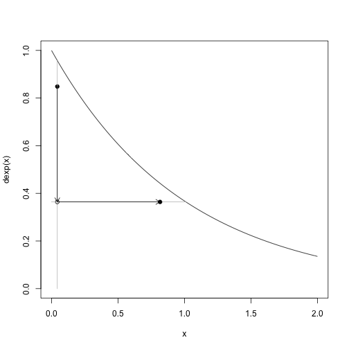
# This code was used step-by-step in class.Here are 9 steps, 10 samples including the intial, of the slice sampler:
# Nine steps
curve(dexp,0,3,ylim=c(0,1))
for (i in 1:9) {
  points(x[i],u[i],pch=19, cex=0.5)
  segments(x[i], u[i], x[i], u[i+1], col="gray")
  segments(x[i], u[i+1], x[i+1], u[i+1], col="gray")
}
points(x[i+1],u[i+1],pch=19, cex=0.5)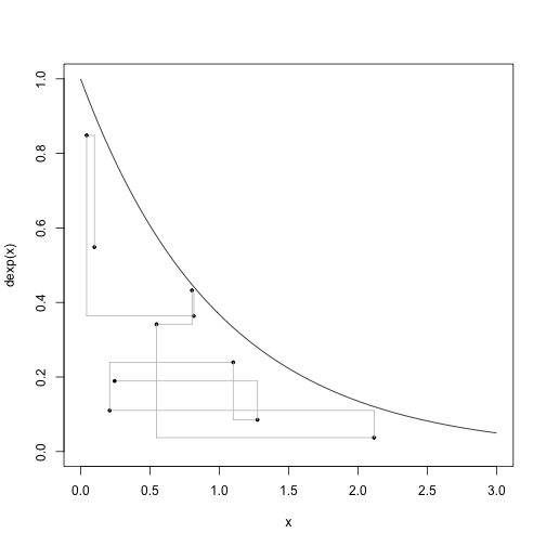
And this is comparing the marginal draws for x to the truth.
hist(slice(1e4, 0.1, dexp, A)$x, freq=F, 100)
curve(dexp, add=TRUE)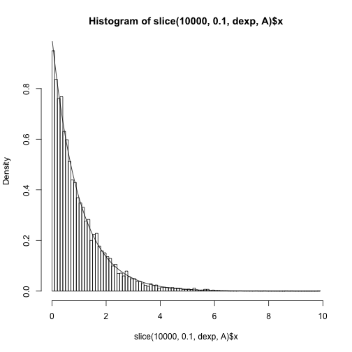
Now I turn to a standard normal distribution where we pretend we cannot invert the density and therefore need another approach. The approach is going to be to use numerical methods to find the interval A (so, again assuming a unimodal target). The magic happens below where the uniroot function is used to find the endpoints of the interval.
A = function(u,xx) {
  c(uniroot(function(x) dnorm(x)-u, c(-10^10,xx))$root,
    uniroot(function(x) dnorm(x)-u, c(xx, 10^10))$root)
}
Run the sampler for a standard normal target.
set.seed(6)
res = slice(10, 0.1, dnorm, A)
x = res$x
u = res$u
This is what one step looks like.
# One step
i = 4
curve(dnorm,-3,3,ylim=c(0,0.5))
points(x[i],u[i],pch=19)
segments(x[i], 0, x[i], dnorm(x[i]), col="gray")
arrows(x[i], u[i], x[i], u[i+1], length=0.1)
points(x[i],u[i+1])
segments(A(u[i+1],x[i])[1],u[i+1],A(u[i+1],x[i])[2],u[i+1],col="gray")
arrows(x[i], u[i+1], x[i+1], u[i+1], length=0.1)
points(x[i+1],u[i+1],pch=19)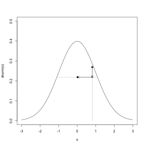
Or 9 steps:
# Nine steps
curve(dnorm,-3,3,ylim=c(0,0.5))
for (i in 1:9) {
  points(x[i],u[i],pch=19, cex=0.5)
  segments(x[i], u[i], x[i], u[i+1], col="gray")
  segments(x[i], u[i+1], x[i+1], u[i+1], col="gray")
}
points(x[i+1],u[i+1],pch=19, cex=0.5)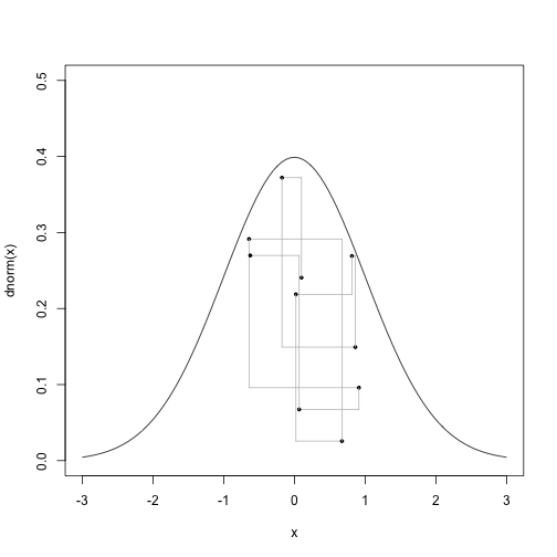
And the fit to the target distribution.
hist(slice(1e4, 0.1, dnorm, A)$x, freq=F, 100)
curve(dnorm, add=TRUE)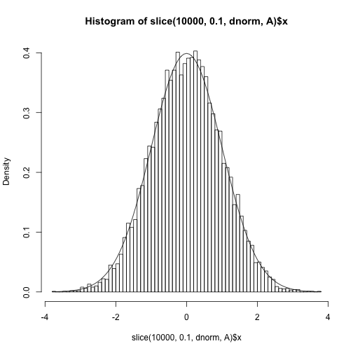
Using an unnormalized density
Slice sampling can also be performed on the unnormalized density.
####
# Standard normal with unnormalized density
set.seed(6)
target = function(x) exp(-x^2/2) # The normalizing factor is 1/sqrt(2pi)
A = function(u,x) {
  x = sqrt(-2*log(u))
  return(c(-x,x))
}

hist(slice(1e4, 0.1, target, A)$x, freq=F, 100)
curve(dnorm, add=TRUE)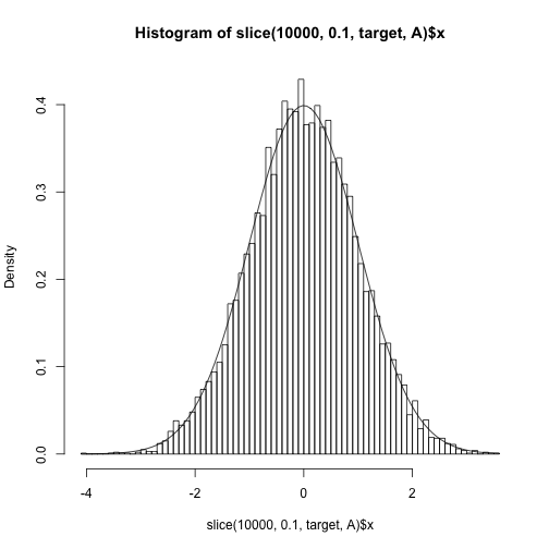
Learning the truncation points
| Here is an alternative version of the slice sampler that samples from a distribution other than uniform. The main purpose of introducing this is in Bayesian inference where the target distribution is the posterior, p(x | y) \propto p(y | x) p(x), and the augmentation is p(u,x)\propto p(x) I(0<u<p(y | x)). So the conditional for x | u is a truncated version of the prior. |
| The truncation points are determined by u<p(y | x) and the truncation points are not assumed to be known. Instead, they are learned through proposed values that are rejected. So, initially we sample from p(x)I(-Inf<0<Inf) (if x has support on the whole real line) and then adjust to p(x)I(LB<x<UB) where LB and UB are updated depending on whether the proposed value that was rejected was larger or smaller than the current value for x. If the proposed value is larger than the current, then UB becomes the proposed value and if it is smaller than LB becomes the proposed value. |
# Slice sampler that learns endpoints
slice2 = function(n,init_x,like,qprior) {
  u = x = rep(NA,n)
  x[1] = init_x
  u[1] = runif(1,0, like(x[1]))

  for (i in 2:n) {
    u[i] = runif(1,0, like(x[i-1]))
    success = FALSE
    endpoints = 0:1
    while (!success) {
      up = runif(1, endpoints[1], endpoints[2])
      x[i] = qprior(up)
      if (u[i]<like(x[i])) {
        success=TRUE
      } else
      {
        # Updated endpoints when proposed value is rejected
        if (x[i]>x[i-1]) endpoints[2] = up
        if (x[i]<x[i-1]) endpoints[1] = up
      }
    }

  }
  return(list(x=x,u=u))
}| This is run on the model y | x ~ N(x,1) and x~N(0,1) and y=1 is observed. The true posterior is N(y/2,1/2). |
res = slice2(1e4, 0.1, function(x) dnorm(x,1), qnorm)

hist(res$x,freq=F,100)
curve(dnorm(x,0.5,sqrt(1/2)), add=TRUE)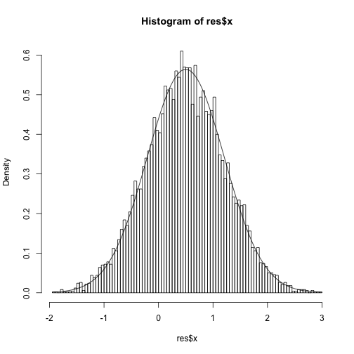
blog comments powered by Disqus