Realizations from a stick breaking representation of a Dirichlet process
This is a quick post looking at realizations of a Dirichlet process via the stick-breaking construction. The Dirichlet process is defined by two parameters: a positive, scalar concentration parameter (alpha) and a base measure (P0).
The stick-breaking construction provides a realization of a Dirichlet process by
- Sampling locations from the base measure.
- Calculating probabilities for each location via breaking a stick of unit length using random Be(1,a) draws.
Given v~Be(1,a), a function to calculate location probabilities is given here.
# Stick-breaking realizations
calc_pi = function(v) {
  n = length(v)
  pi = numeric(n)
  cumv = cumprod(1-v)
  pi[1] = v[1]
  for (i in 2:n) pi[i] = v[i]*cumv[i-1]
  pi
}
A visualization of the stick-breaking process is given here for the first five probabilities. (Anybody know how to make this figure not have so much white space? I tried par(fin=c(5,1)) but that didn’t work.)
par(mar=rep(0,4))
plot(0,0,type='n', xlim=c(0,1), ylim=c(-0.31,0.31), axes=F, xlab='', ylab='')
segments(0,0,1,0)
wd = 0.2
segments(c(0,1),-wd,c(0,1),wd)
wd = wd/1.1

set.seed(9)
pi = calc_pi(rbeta(5,1,10))
cpi = cumsum(pi)
segments(cpi, -wd, cpi, wd)
text(c(0,1),-.3,c(0,1))

midpoint = function(x) {
  n = length(x)
  mp = numeric(n-1)
  for (i in 2:n) mp[i-1] = mean(x[c(i-1,i)])
  mp
}
mp = midpoint(c(0,cpi,1))
text(mp, -0.3, expression(pi[1],pi[2],pi[3],pi[4],pi[5],...))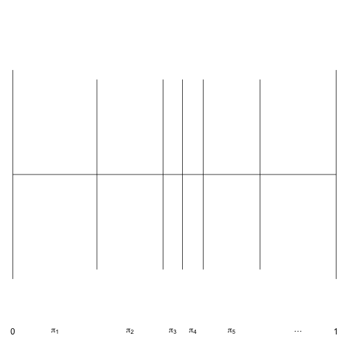
Notice that the probabilities (widths of the intervals) is not strictly decreasing, although the probabilities are stochastically decreasing.
Now, we look at random realizations from this DP which involve random draws from the base measure (rP0) and particle weights given by the stick-breaking process. A function to perform this is given below with a function to plot the results. Note that the stick-breaking construction requires an infinite number of locations and weights, but this is truncated in the function below to H components. One rationale for doing so is that the remaining probably is extremely small.
rdp = function(alpha,rP0,H=1e4) {
  theta = rP0(H)
  v = rbeta(H, 1, alpha)
  pi = calc_pi(v)
  return(list(theta=theta,v=v,pi=pi))
}

plot_rdp = function(rdp,...) {
  plot(rdp$theta,rdp$pi,type="h",...)
}
The function below can be used to visualize realizations from the DP. For simplicity, I have used a standard normal as the base measure. Feel free to run this a few times to get a sense for what the realizations look like.
par(mar=rep(1,4))
plot_rdp(rdp(1,rnorm))
curve(dnorm, col="red", lwd=2, add=TRUE)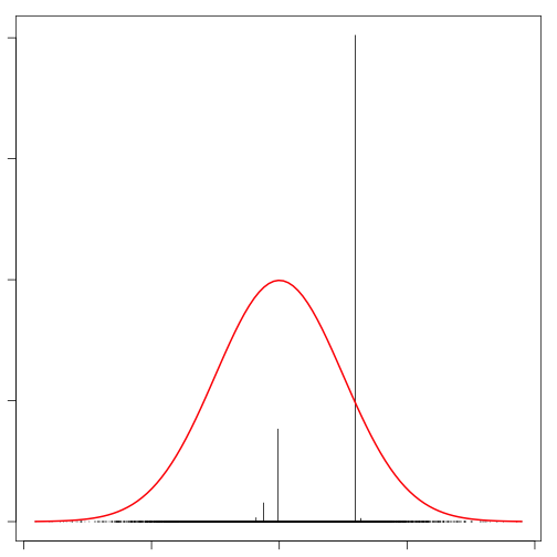
When the concentration parameter is relatively small, a realization from the DP does not look very much like the base measure. Increasing the concentration parameter will result in samples that appear much more like the base measure once they are binnned. Here we use a weighted histogram to bin the samples. The result looks much more like the base measure.
suppressMessages(library(weights,quietly=TRUE))## Error in library(weights, quietly = TRUE): there is no package called 'weights'plot_hist = function(rdp,...) {
wtd.hist(rdp$theta, weight=rdp$pi,...)
}
# Large alpha looks like base measure
plot_hist(rdp(1e5,rnorm), 100, freq=FALSE)## Error in wtd.hist(rdp$theta, weight = rdp$pi, ...): could not find function "wtd.hist"curve(dnorm, col="red", lwd=2, add=TRUE)## Error in plot.xy(xy.coords(x, y), type = type, ...): plot.new has not been called yetblog comments powered by Disqus