Leroux CAR using CARBayes
library("CARBayes")

set.seed(20171109)
sessionInfo()
## R version 3.4.1 (2017-06-30)
## Platform: x86_64-apple-darwin15.6.0 (64-bit)
## Running under: OS X El Capitan 10.11.6
##
## Matrix products: default
## BLAS: /System/Library/Frameworks/Accelerate.framework/Versions/A/Frameworks/vecLib.framework/Versions/A/libBLAS.dylib
## LAPACK: /Library/Frameworks/R.framework/Versions/3.4/Resources/lib/libRlapack.dylib
##
## locale:
<<<<<<< Updated upstream
## [1] en_US.UTF-8/en_US.UTF-8/en_US.UTF-8/C/en_US.UTF-8/en_US.UTF-8
=======
## [1] LC_CTYPE=en_US.UTF-8 LC_NUMERIC=C LC_TIME=en_US.UTF-8 LC_COLLATE=en_US.UTF-8 LC_MONETARY=en_US.UTF-8 LC_MESSAGES=en_US.UTF-8 LC_PAPER=en_US.UTF-8
## [8] LC_NAME=C LC_ADDRESS=C LC_TELEPHONE=C LC_MEASUREMENT=en_US.UTF-8 LC_IDENTIFICATION=C
>>>>>>> Stashed changes
##
## attached base packages:
## [1] stats graphics grDevices utils datasets methods base
##
## other attached packages:
<<<<<<< Updated upstream
## [1] CARBayes_5.0 Rcpp_0.12.13 bindrcpp_0.2 dplyr_0.7.4 xtable_1.8-2
## [6] Hmisc_4.0-3 Formula_1.2-2 survival_2.41-3 lattice_0.20-35 MCMCpack_1.4-0
## [11] MASS_7.3-47 coda_0.19-1 dlm_1.1-4 ggplot2_2.2.1.9000 plyr_1.8.4
## [16] knitr_1.17
##
## loaded via a namespace (and not attached):
## [1] deldir_0.1-14 gtools_3.5.0 assertthat_0.2.0 digest_0.6.12
## [5] truncnorm_1.0-7 R6_2.2.2 backports_1.1.1 acepack_1.4.1
## [9] MatrixModels_0.4-1 evaluate_0.10.1 spam_2.1-1 highr_0.6
## [13] rlang_0.1.2 lazyeval_0.2.0 spdep_0.6-15 gdata_2.18.0
## [17] data.table_1.10.4 SparseM_1.77 gmodels_2.16.2 rpart_4.1-11
## [21] Matrix_1.2-11 checkmate_1.8.4 labeling_0.3 splines_3.4.1
## [25] stringr_1.2.0 foreign_0.8-69 htmlwidgets_0.9 munsell_0.4.3
## [29] compiler_3.4.1 shapefiles_0.7 pkgconfig_2.0.1 base64enc_0.1-3
## [33] mcmc_0.9-5 htmltools_0.3.6 nnet_7.3-12 expm_0.999-2
## [37] tibble_1.3.4 gridExtra_2.3 htmlTable_1.9 matrixcalc_1.0-3
## [41] grid_3.4.1 nlme_3.1-131 gtable_0.2.0 magrittr_1.5
## [45] scales_0.5.0.9000 stringi_1.1.5 reshape2_1.4.2 LearnBayes_2.15
## [49] sp_1.2-5 latticeExtra_0.6-28 boot_1.3-20 CARBayesdata_2.0
## [53] RColorBrewer_1.1-2 tools_3.4.1 glue_1.1.1 colorspace_1.3-2
## [57] cluster_2.0.6 dotCall64_0.9-04 bindr_0.1 quantreg_5.33
=======
## [1] knitr_1.17 ggplot2_2.2.1 bindrcpp_0.2 dplyr_0.7.4 CARBayes_5.0 Rcpp_0.12.13 MASS_7.3-47
##
## loaded via a namespace (and not attached):
## [1] gtools_3.5.0 spam_2.1-1 splines_3.4.0 lattice_0.20-35 colorspace_1.3-2 expm_0.999-2 htmltools_0.3.6 yaml_2.1.14 MCMCpack_1.4-0 rlang_0.1.2
## [11] foreign_0.8-69 glue_1.1.1 sp_1.2-5 bindr_0.1 plyr_1.8.4 stringr_1.2.0 MatrixModels_0.4-1 dotCall64_0.9-04 CARBayesdata_2.0 munsell_0.4.3
## [21] gtable_0.2.0 coda_0.19-1 evaluate_0.10.1 labeling_0.3 SparseM_1.77 quantreg_5.33 spdep_0.6-13 highr_0.6 backports_1.1.0 scales_0.4.1
## [31] gdata_2.18.0 truncnorm_1.0-7 deldir_0.1-14 mcmc_0.9-5 digest_0.6.12 stringi_1.1.5 gmodels_2.16.2 grid_3.4.0 rprojroot_1.2 tools_3.4.0
## [41] LearnBayes_2.15 magrittr_1.5 lazyeval_0.2.0 tibble_1.3.4 tidyr_0.6.3 pkgconfig_2.0.1 Matrix_1.2-10 shapefiles_0.7 matrixcalc_1.0-3 assertthat_0.2.0
## [51] rmarkdown_1.6 R6_2.2.2 boot_1.3-20 nlme_3.1-131 compiler_3.4.0
>>>>>>> Stashed changesUsing the data from this post, we will utilize the intrinsic CAR prior to account for spatial association.
load("data/spatial20171108.rda")
head(d)
## x.easting x.northing Y_normal Y_pois trials Y_binom x1 x2
## 1 1 1 -1.28 1 10 2 -2.01 0.00
## 2 2 1 1.49 4 10 10 0.55 0.38
## 3 3 1 1.36 3 10 9 0.10 0.79
## 4 4 1 0.55 2 10 7 0.08 -0.14
## 5 5 1 0.89 0 10 6 -0.54 1.13
## 6 6 1 0.02 2 10 3 0.35 -0.84Build a neighborhood structure based on 4 nearest neighbors, i.e. cardinal directions.
n <- nrow(d)
distance <- as.matrix(dist(d[,c("x.easting","x.northing")]))

# Proximity matrix
W              <- matrix(0, nrow = n, ncol = n)
W[distance==1] <- 1 image(W)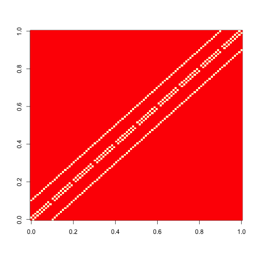
Normal model
system.time(
  mn <- S.CARleroux(formula  = Y_normal ~ x1 + x2,
                   family   = "gaussian",
                   data     = d,
                   W        = W,
                   burnin   = 20000,
                   n.sample = 100000,
                   verbose  = FALSE)
)
## user system elapsed
<<<<<<< Updated upstream
## 46.585 3.461 58.758
=======
## 34.686 0.021 34.686
>>>>>>> Stashed changesmn##
## #################
## #### Model fitted
## #################
## Likelihood model - Gaussian (identity link function)
## Random effects model - Leroux CAR
## Regression equation - Y_normal ~ x1 + x2
## Number of missing observations - 0
##
## ############
## #### Results
## ############
## Posterior quantities and DIC
##
## Median 2.5% 97.5% n.sample % accept n.effective Geweke.diag
## (Intercept) 0.6246 0.6007 0.6482 80000 100.0 71227.6 1.1
## x1 0.9858 0.9454 1.0261 80000 100.0 9705.5 1.2
## x2 0.9855 0.9415 1.0288 80000 100.0 10652.6 -1.4
## nu2 0.0116 0.0028 0.0339 80000 100.0 1707.9 -1.2
## tau2 0.0941 0.0443 0.1462 80000 100.0 2796.8 0.8
## rho 0.7965 0.4777 0.9762 80000 46.4 8039.8 -1.8
##
## DIC = -85.85667 p.d = 75.64239 Percent deviance explained = 99.85Binomial model
system.time(
  mb <- S.CARleroux(formula  = Y_binom ~ x1 + x2,
                   family   = "binomial",
                   data     = d,
                   trials   = d$trials,
                   W        = W,
                   burnin   = 20000,
                   n.sample = 100000,
                   verbose  = FALSE)
)
## user system elapsed
<<<<<<< Updated upstream
## 41.939 3.307 54.727
=======
## 45.429 0.000 45.336
>>>>>>> Stashed changesmb##
## #################
## #### Model fitted
## #################
## Likelihood model - Binomial (logit link function)
## Random effects model - Leroux CAR
## Regression equation - Y_binom ~ x1 + x2
## Number of missing observations - 0
##
## ############
## #### Results
## ############
## Posterior quantities and DIC
##
## Median 2.5% 97.5% n.sample % accept n.effective Geweke.diag
## (Intercept) 0.7605 0.6058 0.9195 80000 46.7 27341.8 0.0
## x1 1.1665 0.9778 1.3660 80000 46.7 16039.1 -1.1
## x2 1.0521 0.8521 1.2629 80000 46.7 16606.4 -0.9
## tau2 0.0066 0.0019 0.0457 80000 100.0 366.7 -2.0
## rho 0.4259 0.0302 0.9046 80000 46.2 2283.1 1.1
##
## DIC = 313.4038 p.d = 3.215662 Percent deviance explained = 48.48Poisson model
system.time(
  mp <- S.CARleroux(formula  = Y_pois ~ x1 + x2,
                   family   = "poisson",
                   data     = d,
                   W        = W,
                   burnin   = 20000,
                   n.sample = 100000,
                   verbose  = FALSE)
)
## user system elapsed
<<<<<<< Updated upstream
## 35.681 3.248 51.700
=======
## 36.443 0.000 36.398
>>>>>>> Stashed changesmp##
## #################
## #### Model fitted
## #################
## Likelihood model - Poisson (log link function)
## Random effects model - Leroux CAR
## Regression equation - Y_pois ~ x1 + x2
## Number of missing observations - 0
##
## ############
## #### Results
## ############
## Posterior quantities and DIC
##
## Median 2.5% 97.5% n.sample % accept n.effective Geweke.diag
## (Intercept) 0.7074 0.5490 0.8576 80000 46.1 3431.2 0.6
## x1 1.0246 0.9068 1.1267 80000 46.1 2395.6 -2.0
## x2 0.8789 0.7599 1.0095 80000 46.1 4629.7 -0.5
## tau2 0.0274 0.0029 0.1610 80000 100.0 321.4 1.7
## rho 0.4391 0.0311 0.9158 80000 46.1 2391.9 1.2
##
## DIC = 384.2647 p.d = 7.403478 Percent deviance explained = 69.31blog comments powered by Disqus