Bayesian logistic regression

This exploration looks at Bayesian logistic regression using Pólya-Gamma latent variables.

Implied priors for a binomial probability

In a binomial model, we have two objective priors that people might argue over: Be(1,1) and Be(1/2,1/2). The former is uniform on the interval (0,1) and the latter is the Jeffreys’ prior, i.e. it is invariant to the transformation used. We also have objective priors that people are happy with for Bayesian regression, namely the joint prior for coefficients and variance is proportional to one divided by the variance. This implies a uniform prior over the whole real line for the coefficients.

When we try to use the regression-style priors in the logistic (or probit) regression, the implied prior on the probability ends up having huge tails at 0 and 1 with little mass anywhere between 0 and 1. This would seem to contradict the objective priors we like for a binomial probability.

The regression-style prior is suggested in the linked paper and here is some code the simulates the implied prior on p. The model here is a mixed effect logistic regression model where beta is the coefficient for the fixed effect and delta are the random effects. Here we are just looking at, for example, one particular observation. But since we have set the long explanatory variable to zero (and thus the impact of the prior for beta is eliminated), all observations are exchangeable and the implied prior on p is the same for all observations.

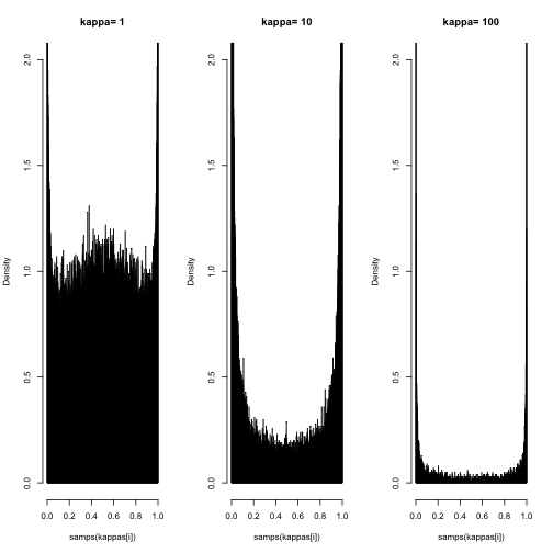
The first function here just creates a sample from the prior suggested in the paper. Formally, the authors take the limit as kappa goes to infinity. We will approximate this by increasing kappa and determining what happens.

p = function(psi) 1/(1+exp(-psi))

samps = function(kappa, 
                 phi.a=1, 
                 phi.b=1, 
                 beta.sigma=100, 
                 x = 0,
                 n=1e5) {
  phi = rgamma(n, phi.a, phi.b)
  sd = 1/sqrt(phi)

  beta = rnorm(n,0,beta.sigma)
  delta = rnorm(n,0,sd)
  m = rnorm(n,0,kappa*sd)
  
  p(m+delta+x*beta)
}

Below are three plots where kappa has increased from 1 to 10 to 100. With kappa=1, the prior looks almost uniform but appears to have a peak near 0 and 1. As kappa is increased this peak gets higher and higher. This implied prior does not seem objective at all.

kappas = 10^c(0:2)
par(mfrow=c(1,length(kappas)))
for (i in 1:length(kappas)) {
  hist(samps(kappas[i]), 1000, freq=F, 
       main=paste("kappa=",kappas[i]), ylim=c(0,2))
}

center

Accept/reject algorithm

This was not discussed in class, but is just a simple example of an accept/reject algorithm to sample a standard normal using a t distribution.

# sample Z~N(0,1) using X~t_df
df = 5
n = 1e6 # number of attempts
c = exp(dnorm(0,log=T)-dt(0,df,log=T))
x = rt(n,df)
lu = log(runif(n))+log(c)+dt(x,df,log=T)
z = x[lu<=dnorm(x,log=T)]

In the plot below is a histogram of the samples with two curves representing the target distribution (normal) and the proposal distribution (t). It appears to do reasonably well although I’m concerned with the slightly higher peak at the mode of the distribution. Is this just due to binning?

hist(z, 100, freq=F)
curve(dnorm, add=T, col=4, lwd=2)
curve(dt(x,df), add=T, col=2, lwd=2, lty=2)
legend("topright",c("normal","t"), col=c(4,2), lty=1:2, lwd=2)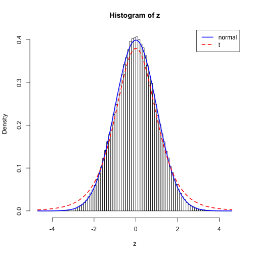

center

I also decided to check the acceptance rate relative to the expected acceptance rate and these don’t seem to quite agree. Do I have a bug somewhere?

length(z)/n # acceptance rate, should be 1/c

## [1] 0.932718

1/c

## [1] 0.9515329