Interweaving Gibbs samplers
This exploration looks at the interweaving sampler of Yu and Meng. The model is Y~N(theta,1+V) with V known and two different data augmentation schemes are considered:
- Sufficient Augmentation: Y~N(Ymis,1), Ymis~N(theta,1)
- Ancillary Augmentation: Y~N(Ymist+theta,1), Ymist~N(0,V)
Ymis and Ymist (Ymis tilde) are the augmentations. The second is named ancillary since the distribution for the augmented data does not depend on the parameter. The first is named sufficient because the full conditional distribution for the parameter, theta, does not depend on the data: theta|Ymis, Yobs ~ N(Ymis, V).
First, we set up the full conditionals for SA:
draw_YmisSA = function(theta, Yobs, V) {
  rnorm(1, (theta+V*Yobs)/(1+V), sqrt(V/(1+V)))
}

draw_thetaSA = function(Ymis, V) {
  rnorm(1, Ymis, V)
}
Next, we set up the full conditionals for AA:
draw_YmistAA = function(theta, Yobs, V) {
  rnorm(1, V*(Yobs-theta)/(1+V), sqrt(V/(1+V)))
}

draw_thetaAA = function(Ymis, Yobs, V) {
  rnorm(1, Yobs-Ymis, 1)
}
We also need the mapping between the two augmentations.
M    = function(Ymis,  theta) Ymis  - theta
Minv = function(Ymist, theta) Ymist + theta
Now, we build a generic MCMC function that will run all of the schemes where AA is the MCMC associated with the ancillary augmentation, SA is the MCMC associated with the sufficient augmentation, ALT is the MCMC where a single iteration is SA followed by AA, and ASIS is the Ancillary-Sufficiency Interweaving Strategy introduced in Yu and Meng.
mcmc = function(input) {
  V      = input$V
  Yobs   = input$Yobs
  n.reps = input$n.reps

  thetas = rep(input$theta0,n.reps)

  scheme = pmatch(input$scheme,c("AA","SA","ALT","ASIS"))

  switch(scheme,
    { # AA
      for (i in 2:n.reps) {
        Ymist     = draw_YmistAA(thetas[i-1],Yobs,V)
        thetas[i] = draw_thetaAA(Ymist,Yobs,V)
      }
    },
    { # SA
      for (i in 2:n.reps) {
        Ymis      = draw_YmisSA(thetas[i-1],Yobs,V)
        thetas[i] = draw_thetaSA(Ymis,V)
      }
    },
    {# ALT
      for (i in 2:n.reps) {
        Ymis      = draw_YmisSA(thetas[i-1],Yobs,V)
        theta     = draw_thetaSA(Ymis,V)
        Ymist     = draw_YmistAA(thetas     ,Yobs,V)
        thetas[i] = draw_thetaAA(Ymist,Yobs,V)
      }
    },
    {# ASIS
      for (i in 2:n.reps) {
        Ymis      = draw_YmisSA(thetas[i-1],Yobs,V)
        theta     = draw_thetaSA(Ymis,V)
        Ymist     = M(Ymis,theta) # This step is different from ALT.
        thetas[i] = draw_thetaAA(Ymist,Yobs,V)
      }
    }
  )


  data.frame(V=V, scheme=input$scheme, theta=thetas)
}
Notice that the only step that is different between ASIS and ALT is the 3rd step where ASIS has a deterministic step while ALT has a sampling step. Yet, as shown in the paper, ASIS leads to independent draws from the posterior while ALT leads to positively correlated draws.
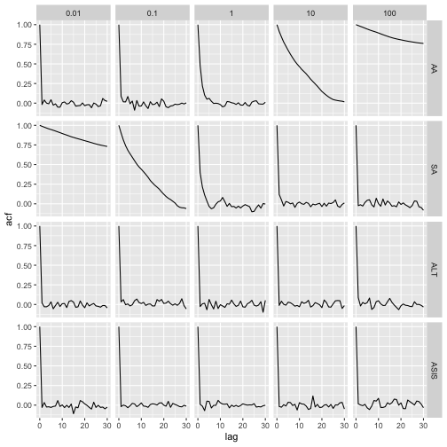
Now let’s look at the autocorrelation in the chains for theta from these different MCMC schemes for various values of V.
library(plyr)
schemes = c("AA","SA","ALT","ASIS")
exp = expand.grid(scheme=factor(schemes,schemes,ordered=TRUE), n.reps=1000,
                  V=10^seq(-2,2), theta0=0, Yobs=0)
out = ddply(exp, .(scheme, V), mcmc, .inform=T)

my_acf = function(x) {
  tmp = acf(x$theta, plot=F)
  data.frame(lag=as.numeric(tmp$lag), acf=as.numeric(tmp$acf))
}
acfs = ddply(out, .(scheme, V), my_acf)

library(ggplot2)
qplot(lag, acf, data=acfs, facets=scheme~V, geom="line")
Notice how AA has high autocorrelation when V is large, SA has high autocorrelation when V is small. Both the ALT and ASIS samplers have low autocorrelation everywhere. The difference between ALT and ASIS is not obvious here, but remember they are essentially the same sampler except ASIS has a deterministic step where ALT has a sampling step and ASIS obtains independent samples from the posterior.
blog comments powered by Disqus