Finite mixtures
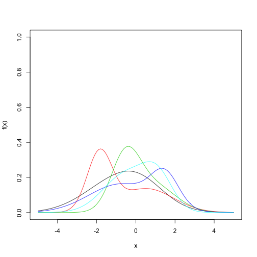
This post looks at finite mixtures of normals. The first bit of code here looks at the flexibility of mixtures of normals. Feel free to change the argument to the plots function to try more mixtures.
library(MCMCpack)## Loading required package: coda##
## Attaching package: 'coda'## The following object is masked _by_ '.GlobalEnv':
##
## mcmc## Loading required package: MASS## ##
## ## Markov Chain Monte Carlo Package (MCMCpack)## ## Copyright (C) 2003-2017 Andrew D. Martin, Kevin M. Quinn, and Jong Hee Park## ##
## ## Support provided by the U.S. National Science Foundation## ## (Grants SES-0350646 and SES-0350613)
## ##dmix = function(M) {
alpha = 1
pi = as.numeric(rdirichlet(1, rep(alpha,M)))
mu = rnorm(M)
sigma = sqrt(rgamma(M,1))
f = function(x) sum(pi*dnorm(x,mu,sigma))
vf = Vectorize(f)
}
plots = function(M) {
plot(0,0, type="n", xlim=c(-5,5), ylim=c(0,1),
xlab="x", ylab="f(x)")
for (i in 1:5) {
f = dmix(M)
curve(f, add=TRUE, col=i)
}
}
plots(2)
We now look at estimating the model using JAGS. This first versions shows identifiability issues that arise due to label switching.
mix = function(M) {
  alpha = 1
  pi = as.numeric(rdirichlet(1, rep(alpha,M)))

  mu = rnorm(M)
  sigma = sqrt(rgamma(M,1))

  return(list(pi=pi,mu=mu,sigma=sigma))
}

rmix = function(n,mix) {
  eta = sample(length(mix$pi), n, replace=TRUE, prob=mix$pi)
  y   = rnorm(n, mix$mu[eta], mix$sigma[eta])
  return(list(eta=eta,y=y))
}

set.seed(1)
M = 2
m = list(pi=c(.4,.6), mu=c(-2,2), sigma=c(1,1))
d = rmix(20, m)

dat = list(M=M, y=d$y, alpha=rep(1,M), n=length(d$y))

library(rjags)
## Error in library(rjags): there is no package called 'rjags'jags_model = "
model {
for (i in 1:n) {
y[i] ~ dnorm(mu[eta[i]], tau[eta[i]])
eta[i] ~ dcat(pi[])
}
for (i in 1:M) {
mu[i] ~ dnorm(0,1)
tau[i] ~ dgamma(1,1)
sigma[i] <- 1/sqrt(tau[i])
}
pi ~ ddirich(alpha)
}"
jm = jags.model(textConnection(jags_model),
data=dat, n.chains=3)## Error in jags.model(textConnection(jags_model), data = dat, n.chains = 3): could not find function "jags.model"update(jm, 100)## Error in update(jm, 100): object 'jm' not foundres = coda.samples(jm, c("mu","sigma","eta","pi"), n.iter=3e3)## Error in coda.samples(jm, c("mu", "sigma", "eta", "pi"), n.iter = 3000): could not find function "coda.samples"plot(res)## Error in xy.coords(x, y, xlabel, ylabel, log): 'x' is a list, but does not have components 'x' and 'y'The non-identifiability can be seen by the observations having the same probability of coming from each component as well as the near identical posteriors for mu and sigma from each component.
In order to make the parameters identified, we order the means using the sort function in JAGS.
# Order the components by their means to make
# the mixture components identifiable
identified_jags_model = "
model {
  for (i in 1:n) {
    y[i] ~ dnorm(mu[eta[i]], tau[eta[i]])
    eta[i] ~ dcat(pi[])
  }

  for (i in 1:M) {
    mu0[i] ~ dnorm(0,1)
    tau[i] ~ dgamma(1,1)
    sigma[i] <- 1/sqrt(tau[i])
  }
  mu[1:M] <- sort(mu0)

  pi ~ ddirich(alpha)
}"

ijm = jags.model(textConnection(identified_jags_model),
                data=dat, n.chains=3)
## Error in jags.model(textConnection(identified_jags_model), data = dat, : could not find function "jags.model"ires = coda.samples(ijm, c("mu","sigma","eta","pi"), n.iter=2e3)## Error in coda.samples(ijm, c("mu", "sigma", "eta", "pi"), n.iter = 2000): could not find function "coda.samples"plot(ires)## Error in plot(ires): object 'ires' not foundblog comments powered by Disqus